Fast Fourier Transform

Discrete Fourier Transform (DFT)

As mentioned before, the Fourier transform of $s(t)$ is

$$S(f) = \int_{-\infty}^{\infty} s(t) e^{-j 2 \pi f t} \, dt$$

In many applications, it's difficult to find the functional form of $s(t)$, and even if it can be found, it's often not possible to find a closed-form solution for the integral. Therefore, in most cases, we use numerical methods to calculate the Fourier transform, with the most common method being the Discrete Fourier Transform (DFT).

Assuming the signal $s(t)$ is sampled at $N$ points within an interval, with values $s_0, s_1, \cdots, s_{N-1}$, its DFT is defined as:

$$S_k = \sum_{n=0}^{N-1} s_n e^{-j\frac{2\pi}{N}nk}$$

Note in the above equation, the value remains unchanged when $k$ increases by $N$, so the main transformation values are $S_0, S_1, \cdots, S_{N-1}$.

Comparing the integral formula with the definition of DFT, we find some similarities. Since DFT deals with sampled signal values limited to $N$ points within an interval, we can consider the $S_k$ values calculated by DFT as approximate sampling values of $S(f)$.

According to the sampling theorem mentioned earlier, if the sampling rate is $f_s$, then the signal frequency that can be restored ranges between [-$f_s/2$, $f_s/2$], divided evenly into $N$ parts, each part size being

$$\Delta f = \frac{f_s/2 - (-f_s/2)}{N} = \frac{f_s}{N} = \frac1{NT}$$

Here, $T$ is the sampling time interval, hence $NT$ is the total time of the entire sampling interval. Some key properties of the DFT mentioned above are summarized as follows:

1. Converts $N$ time sampling points $s_0, s_1, \cdots, s_{N-1}$ into $N$ frequency sampling points $S_0, S_1, \cdots, S_{N-1}$, where $S_k$ is periodic with a period of $N$.
2. If the sampling rate is $f_s$, the highest frequency value that can be determined is $f_s/2$.
3. The interval between sampling frequencies is the reciprocal of the total sampling time length.

DFT has many other important properties, three of which are listed below:

1. DFT operation is linear, i.e., DFT($ax+by$) = $a$ DFT($x$) + $b$ DFT($y$).
2. If $s_n$ is real, then $S_k = S^*_{-k} = S^*_{N-k}$, where * denotes the complex conjugate.
3. Based on the DFT formula above, the inverse DFT is obtained as follows:

$$s_n = \sum_{k=0}^{N-1} S_k e^{j\frac{2\pi}{N}nk}$$

Fast Fourier Transform (FFT)

In calculating the DFT, many symmetries and conjugate properties in the formula can be used to speed up the computation process. This method of fast computation is known as the Fast Fourier Transform, abbreviated as FFT. FFT has various computational forms, but essentially, it is an algorithm for quickly calculating the DFT. The inverse of FFT is called the Inverse FFT, or IFFT.

In signal processing, we often use the Fast Fourier Transform (FFT) to calculate its spectrum. When using FFT, remember the following key points:

1. Assuming the signal segment used for analysis has $N$ points, and its sampling interval is $T$, then the total length of this signal segment is $NT$, and the sampling rate is $f_s=1/T$.

2. According to the sampling theorem, the observable frequency range is $[-f_M,f_M]$, where $f_M=f_s/2$.

3. $N$ time-domain points become $N$ frequency-domain points after FFT, hence the frequency resolution, or the interval between adjacent frequency points, is $2f_M/N = f_s/N = 1/(NT)$. Simply put, the reciprocal of the total sampling time is the distance between frequency sampling points, which is the frequency resolution.

4. Remember half of the sampling rate is the maximum observable frequency; the reciprocal of the total sampling length is the frequency resolution.

5. For real functions, after performing FFT, the values for positive and negative frequencies will be complex conjugates of each other.

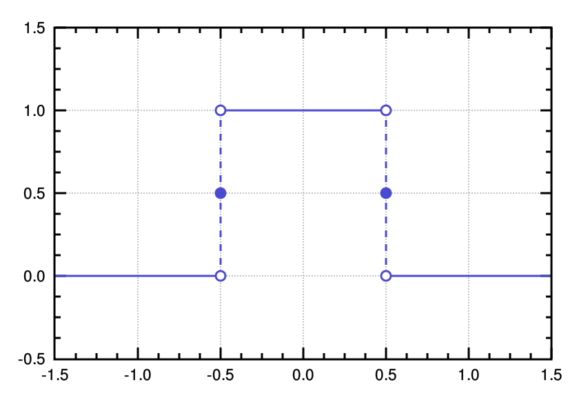
Now, let's observe the spectrum of the hat function. The graph of the rect(t) function is as follows:

The steps to observe its spectrum using MATLAB/Octave are as follows:

1. Assuming the sampling range is from -1.5 to 1.5, taking a point every 0.1, calculate the time-domain signal:

t1 = -1.5:0.1:-0.6;
t2 = -0.4:0.1:0.4;
t3 =  0.6:0.1:1.5;
t = [t1 -0.5 t2 0.5 t3];
s = [zeros(size(t1)) 0.5 ones(size(t2)) 0.5 zeros(size(t3))];
plot(t, s);

This code snippet is a bit cumbersome but easy to understand. Run it to see if the result is correct.

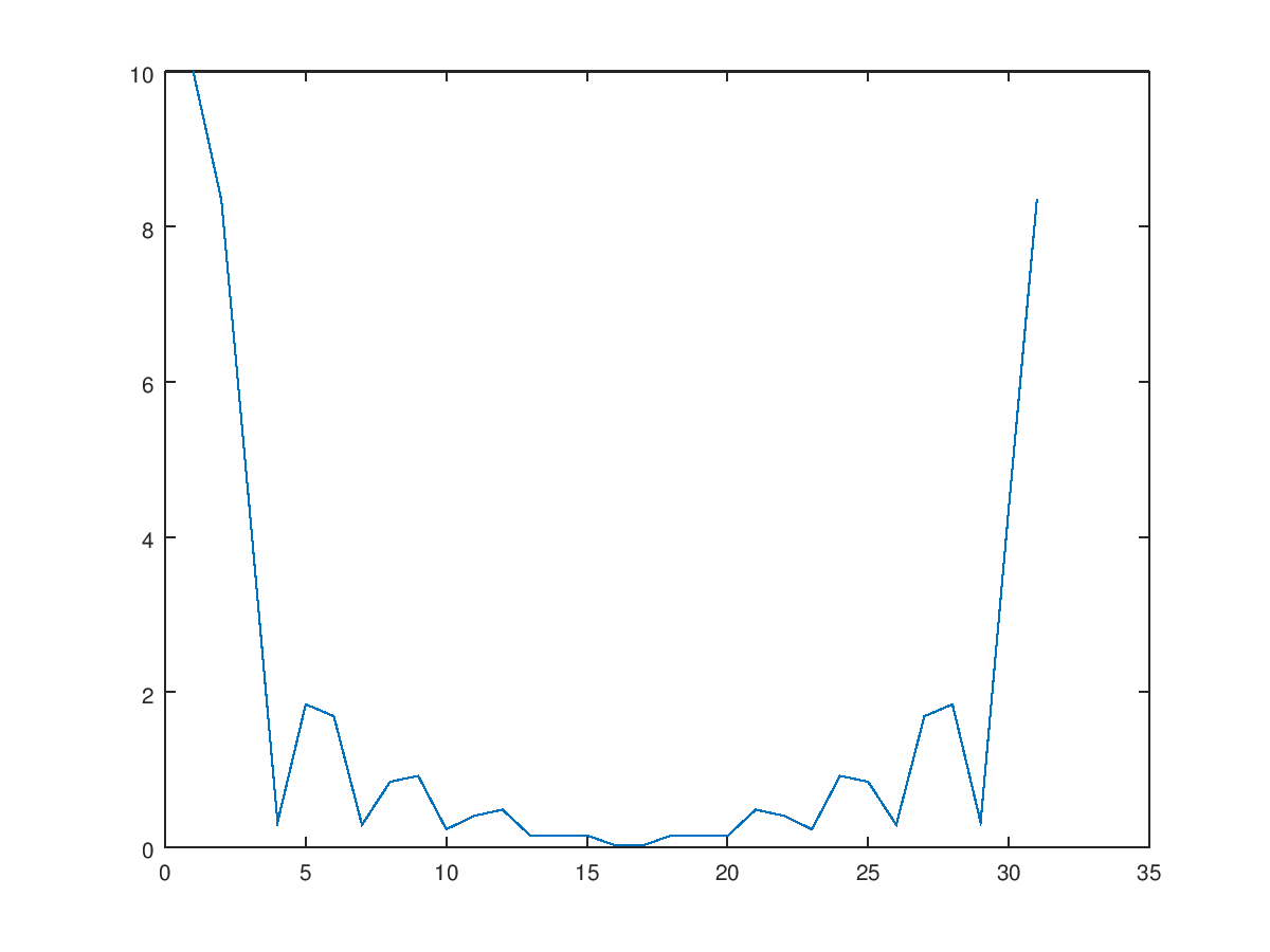
2. To calculate the spectrum, directly use the fft function to transform the above time-domain signal to the frequency domain. Note that the result will be complex, and we first observe its amplitude.

sf = fft(s);
plot(abs(sf));

Note that in the above program, when plotting, only the y-axis is provided, the x-axis will be the number of points, resulting in the following:

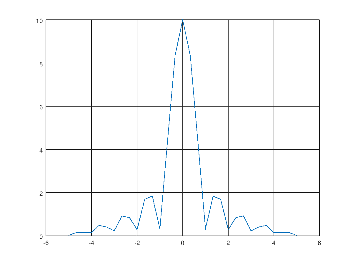
3. As mentioned earlier, for the FFT of a real function, the positive and negative frequencies will be complex conjugates of each other. Actually, in the graph we see now, the right half should be moved to the negative side. MATLAB has a fftshift function that does just that. Additionally, the maximum frequency is half the sampling rate=5, the interval is the reciprocal of the total length=1/3, we need to add the x-axis (frequency) back.

sf = fft(s);
sf = abs(fftshift(sf));
f = -5:1/3:5;
plot(f, sf);
grid on;

Finally, the corrected graph is obtained as shown below, which is the amplitude of the sinc function.

The complete code is as follows:

t1 = -1.5:0.1:-0.6;
t2 = -0.4:0.1:0.4;
t3 =  0.6:0.1:1.5;
t = [t1 -0.5 t2 0.5 t3];
s = [zeros(size(t1)) 0.5 ones(size(t2)) 0.5 zeros(size(t3))];
sf = fft(s);
sf = abs(fftshift(sf));
f = -5:1/3:5;
plot(f, sf);
grid on;

Exercise 4

The spectrum graph above does not look very smooth. Please modify the program's parameters to make the plotted spectrum smoother.