Sampling Theorem

Signal and Its Spectrum

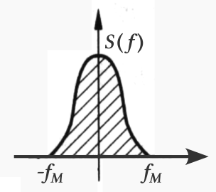
We assume that the signal to be processed is a real function $s(t)$ with its spectrum $S(f)$, and assume that the maximum frequency component of $S(f)$ does not exceed $f_M$. Note that the spectrum of a real function is basically symmetric about the y-axis, as shown in the figure below:

$s(t)$'s spectrum $S(f)$

Mathematical Expression of Sampling

As mentioned earlier, to transition from analog to digital signals, the process generally involves sampling and quantization, where quantization is irreversible and introduces what is called quantization noise.

Let's now talk about sampling.

Assuming the signal is $s(t)$, sampled every $T$ time, the sampling result is $s_n = s(nT)$. Mathematically, we can imagine that the sampling method is equivalent to multiplying the original signal $s(t)$ by a comb function, which is $\text{Ш}_T(t)s(t)$, as shown in the figure below:

Sampling the $s(t)$ function

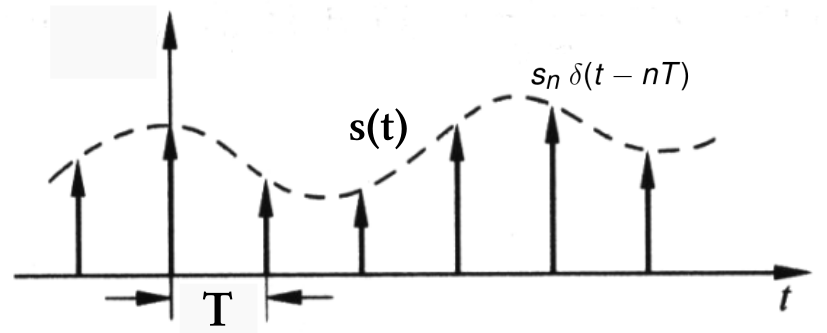
We don't need to worry about the problem of the $\delta$ function approaching $\infty$; just focus on the coefficient before the $\delta$ function.

Spectrum After Sampling

After sampling the signal, let's look at its Fourier transform, that is, the spectrum after sampling. According to the content described earlier:

$$\begin{align*} \mathcal{F}\{\text{Ш}_T(t)s(t)\} &= \mathcal{F}\{\text{Ш}_T(t)\} * \mathcal{F}\{s(t)\} \\ &= \frac{1}{T}\text{Ш}_{\frac{1}{T}}(f) * S(f) \end{align*}$$

Since the $\text{Ш}_{1/T}(f)$ function consists of a series of $\delta$ functions, and when a $\delta$ function convolves with any function, it remains the same function but shifts its center to the center of the $\delta$ function, i.e.,

$$\begin{align*} \text{Ш}_{\frac{1}{T}}(f) * S(f) &= \sum_{n=-\infty}^{\infty} \delta(f-n/T) * S(f) \\ &= \sum_{n=-\infty}^{\infty} S(f-n/T) \end{align*}$$

This results in the following spectrum after sampling (amplitude not considered for now):

$s(t)$'s spectrum after sampling

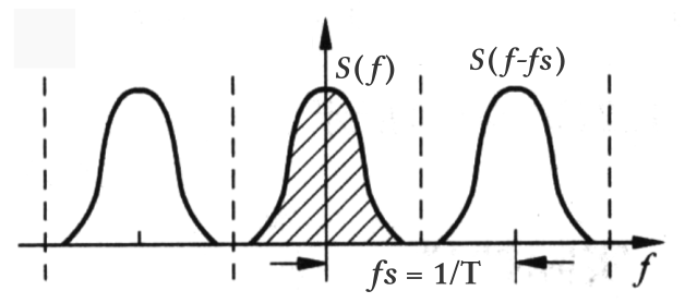
Note that the above figure assumes $f_s > 2f_M$, so there is no overlap between the repeated spectrums. If $f_s < 2f_M$, the repeated spectrums would overlap.

Signal Restoration

If $f_s > 2f_M$, meaning there is no overlap between the repeated spectrums, we can take the middle slanted part of the spectrum as the signal we want to restore. Since the spectrum of the signal is completely the same, the signal itself is also identical. In other words, theoretically, it is possible to restore the original signal from the sampling result. The rate $f_s=2f_M$ is called the Nyquist sampling rate and the corresponding frequency $f_M$ is called the Nyquist frequency.

The restoration method, in terms of the frequency domain, is to multiply the sampled spectrum by a hat function, which is equivalent to low-pass filtering the signal, i.e., only retaining the middle slanted spectrum region and filtering out other frequency areas. Mathematically, this can be represented as (amplitude not considered for now):

$$(\sum_{n=-\infty}^{\infty} S(f-n/T))\ \Pi(f/f_s) = S(f)$$

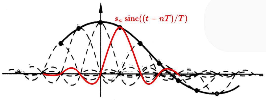
Alternatively, from the time domain perspective, performing the inverse Fourier transform of the above equation results in the time-domain signal. Since multiplication in the frequency domain translates to convolution in the time domain, and the inverse transform of the hat function is the sinc function, the time-domain signal can be expressed as (amplitude not considered for now):

$$\begin{align*} \hat{s}(t) &= (\text{Ш}_T(t)s(t)) * \text{sinc}(f_st) \\ &= \left(\sum_{n=-\infty}^{\infty} s_n\delta(t-nT)\right) * \text{sinc}(f_st) \\ &= \sum_{n=-\infty}^{\infty} s_n\ \text{sinc}(f_s(t-nT))\\ &= \sum_{n=-\infty}^{\infty} s_n\ \text{sinc}((t-nT)/T) \end{align*}$$

The result is shown in the figure below, equivalent to placing a scaled sinc function at each sampling point, where the sinc function has a value of 1 at the sampling position and 0 at other sampling positions. For this reason, the sinc function is sometimes also called the sampling function.

Time-domain equivalent diagram for signal restoration

Exercise 3

1. The content above assumes that the signal bandwidth is limited. Is this assumption reasonable in the real physical world? Please share your views and reasons.
2. In the reasoning process above, it's assumed that the sampling rate is more than twice the signal's highest frequency. What would happen if the actual sampling rate is less than twice the signal's highest frequency?