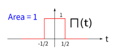
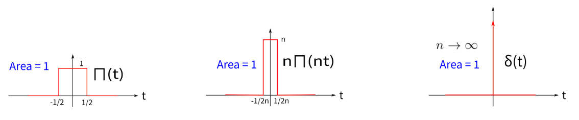
Some Common Functions

rect Function

The rect(t) function is defined as follows:

$$\text{rect}(t) = \begin{cases} 1, & \text{if } |t| < \frac{1}{2} \\ \frac{1}{2}, & \text{if } |t| = \frac{1}{2} \quad (\text{optional condition}) \\ 0, & \text{if } |t| > \frac{1}{2} \end{cases}$$

Its graph is shown below. Since its shape resembles a hat, we sometimes also call it the hat function $\Pi(t)$：

rect(t)

sinc Function

The sinc(t) function is defined as follows:

$$\text{sinc}(t) = \begin{cases} \frac{\sin(\pi t)}{\pi t}, & \text{if } t \neq 0 \\ 1, & \text{if } t = 0 \end{cases}$$

Its graph is shown below:

sinc(t)

Note: $\mathcal{F}\{\Pi(t)\} = \text{sinc}(f)$, $\mathcal{F}\{\text{sinc}(t)\} = \Pi(f)$, they are Fourier transform pairs of each other.

$\delta$ Function

The $\delta(t)$ function is defined as

$$\delta(t) = \lim_{\epsilon \to 0}\ \frac{1}{2\epsilon}\ \text{rect}\left(\frac{t}{2\epsilon}\right)$$

Here, $\text{rect}(t)$ is the rectangular function, which is 1 when $-\frac{1}{2} \leq t \leq \frac{1}{2}$ and 0 otherwise, also denoted as $\Pi(t)$. As $\epsilon$ approaches 0, the width of the rectangular function also approaches 0, and its height approaches $\infty$, but still maintains its integral value as 1, as shown in the following figure:

one representation of $\delta(t)$ function

The $\delta(t)$ function has many important properties and applications, here are a few that will be used in this unit:

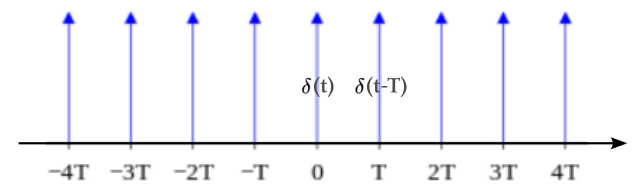
$$\mathcal{F}\{\delta(t)\} = 1$$

$$\mathcal{F}\{1\} = \delta(f)$$

$$\mathcal{F}\{e^{j2\pi f_0t} \} = \delta(f-f_0)$$

$$\begin{align*} f(t) * \delta(t-t_0) &= \int_{-\infty}^{\infty} f(t-\tau) \delta(\tau - t_0) \, d\tau \\ &= f(t-t_0) \end{align*}$$

comb Function

The comb function is defined as follows:

$$\text{comb}_T(t) = \sum_{n=-\infty}^{\infty} \delta(t - nT)$$

Or it can be abbreviated as $\text{Ш}_T(t)$, illustrated below:

$\text{Ш}_T(t)$ function

$\text{Ш}_T(t)$ is a periodic function, and its Fourier series coefficients $c_n=1/T$ can be derived, hence

$$\text{Ш}_T(t) = \sum_{n=-\infty}^{\infty} \frac1T\ e^{j 2 \pi nt/T}$$

Further derivation leads to:

$$\begin{align*} \mathcal{F}\{\text{Ш}_T(t)\} &= \frac{1}{T} \sum_{n=-\infty}^{\infty} \delta(f-n/T) \\ &= \frac{1}{T}\ \text{Ш}_{\frac{1}{T}}(f) \end{align*}$$

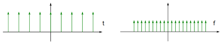
Therefore, the Fourier transform of the comb function remains a comb function, but the spacing between $delta$ functions is inversely proportional in the time and frequency domains, and their heights also change, as illustrated below:

Fourier transform of $\text{Ш}_T(t)$

Exercise 2

The explanation on this page does not detail the derivation process in many places. Please use generative AI to find the derivation process and carefully check to ensure the derivation is correct. You can copy down the process or directly share the interactive link of the generative AI.