Drawing Fourier Series

Assuming the function $s(x)$ is defined on the interval $[x_0, x_0+P]$, it was mentioned earlier that $s(x)$ can be represented as the sum of its Fourier series:

$$s(x) = \frac{a_0}{2} + \sum_{n=1}^{\infty} (a_n\cos(\frac{2\pi n x}{P}) + b_n\sin(\frac{2\pi n x}{P})),$$

where

$$a_n = \frac{2}{P}\int_{x_0}^{x_0+P} s(x)\cos(\frac{2\pi n x}{P})\ dx$$

$$b_n = \frac{2}{P}\int_{x_0}^{x_0+P} s(x)\sin(\frac{2\pi n x}{P})\ dx$$

$a_n$ and $b_n$ are the $n^{th}$ harmonic coefficients.

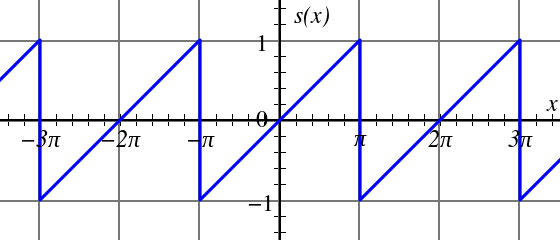
Next, we will use Octave to observe a sawtooth wave, calculate the coefficients of its Fourier series, then sum up the components of $N$ harmonics and compare it with the original waveform. The wave function $s(x)$ used here is as follows:

Its Fourier series can be calculated as:

$$s(x) = \frac{2}{\pi}\sum_{n=1}^{\infty}\frac{(-1)^{n+1}}{n}\sin(nx)$$

The steps of the program are as follows:

1. MATLAB has a sawtooth function that can directly draw a sawtooth waveform. The sawtooth function is defined in the Signal Processing Toolbox. If using MATLAB, ensure this toolbox is correctly installed; if using Octave, then the signal package can be used. For installing Octave packages in Windows, refer to the official website. For Ubuntu, use the following command to install:

   sudo apt-get install octave-signal
   

2. In Octave, first use the pkg load signal command to load the signal package. Then, you can use the sawtooth function (use help sawtooth to view the usage of this function). Try using the following command to draw a sawtooth function graph:

   t = -8:0.1:8;
   s = sawtooth(t-pi); % sawtooth's default period is 2*pi, with a turn at 0
   plot(t,s);
   grid on; % draw grid lines
   

   Observe if the waveform is correct.

3. Draw a partial sum of the series.

   N = 5; % number of terms
   sgn = 1; % used for alternating signs, the first term is positive
   t = -8:0.1:8;
   fs = zeros(size(t)); % set fs to the same dimension as t, all zeros
   for n = 1:N % from 1 to N
   fs = fs + 2*sgn*sin(n*t)/(n*pi); % add one term
   sgn = sgn * -1; % change sign
   end
   plot(t,fs); % plot the graph
   

   Observe the synthesized waveform.

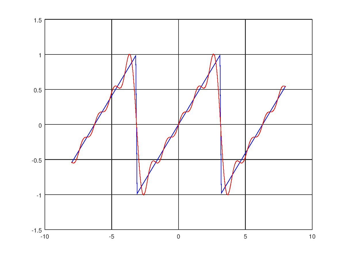
4. Finally, plot both waveforms together, as shown in the following code:

   N = 5;
   t = -8:0.1:8;
   sgn = 1;
   s = sawtooth(t-pi); % sawtooth's default period is 2 pi, with a turn at 0
   fs = zeros(size(s));
   for n = 1:N
   fs = fs + 2*sgn*sin(n*t)/(n*pi);
   sgn = sgn * -1;
   end
   plot(t,s,'b',t,fs,'r');
   grid on; % draw grid lines
   

   The result after execution is as follows:

   

In the above program, we already know the coefficients of $a_n$ and $b_n$ for the Fourier series of $s(x)$. For other functions, it might take a lot of time to calculate. In practice, Octave has a Symbolic Math Toolbox that can assist in symbolic operations. If using Octave, install the symbolic package with the following command:

sudo apt-get install octave-symbolic

Then, use pkg load symbolic to load the package for use. For example, for $f(x)=x^2$, assuming it's defined in the interval $[-\pi,\pi]$, you can calculate the coefficients $a_n$ as follows:

pkg load symbolic
syms x n; % x, n as symbols
f = x^2; % f(x) = x^2
an = int(f*cos(n*x), x, -pi, pi) / pi; % calculate the definite integral value

Exercise 3

Octave has a square function that can be used to draw square wave functions (check with help square). Please calculate the Fourier series of a square wave (you can also look it up online or use the symbolic package for calculation), then use a program to draw the square wave and its partial Fourier series sum. You can define the period and amplitude of the square wave yourself.