Basic Syntax of Octave

Here we introduce some basic programming syntax of Octave. For those who want to delve deeper, it's recommended to borrow MATLAB related books for study.

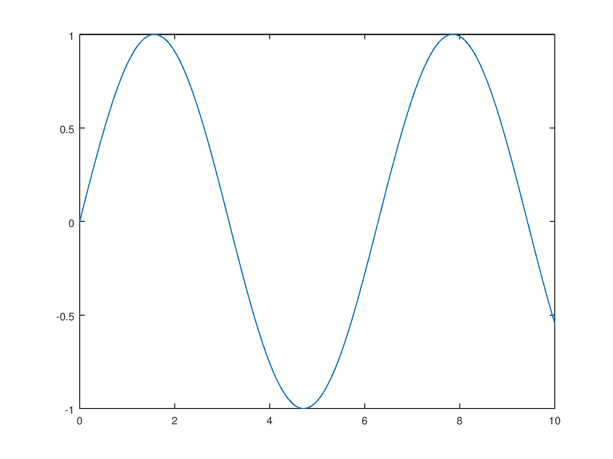
1. Plot the sin(t) function graph

   % The percentage symbol is for comments. If you don't add a semicolon after the expression, it will display the result.
   t=0:0.01:10;   % Generates a 1D matrix from 0, with an interval of 0.01, up to 10
   x=sin(t);      % Calculates the sin function values of t (each element calculated), result is still a 1D matrix
   plot(t,x);     % t is the x-axis, x is the y-axis, draw the graph for t=0:0.01:10;
   

   The result is as follows:

   

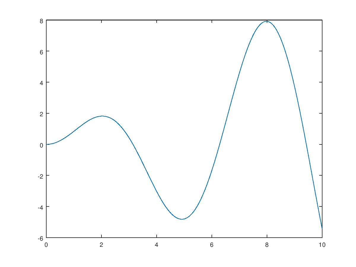
2. Plot the t*sin(t) function graph

   Basically, MATLAB treats each variable as a matrix and allows for addition, subtraction, multiplication, and division, but all operations are done in matrix form. If you want to perform element-wise operations within matrices, you can add a period before the operator.

   t=0:0.01:10;  % Generates a 1D matrix from 0, with an interval of 0.01, up to 10
   x=t.*sin(t);  % Element-wise calculation of t multiplied by the sin function values
   plot(t,x);    % t is the x-axis, x is the y-axis, draw the graph
   

   The result is as follows:

   

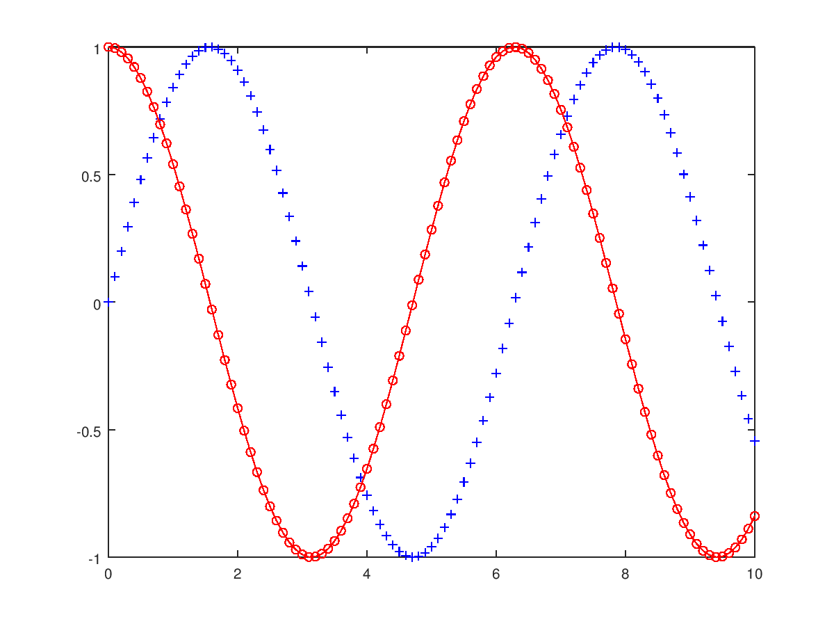
3. Plot multiple graphs

   Plot both sin(t) and cos(x) graphs together with simple styles:

   t=0:0.1:10;
   x1=sin(t);
   x2=cos(x);
   plot(t,x1,'+b',t,x2,'o-r');     % b: blue, r: red, -: line, +o: points
   

   The result is as follows:

   

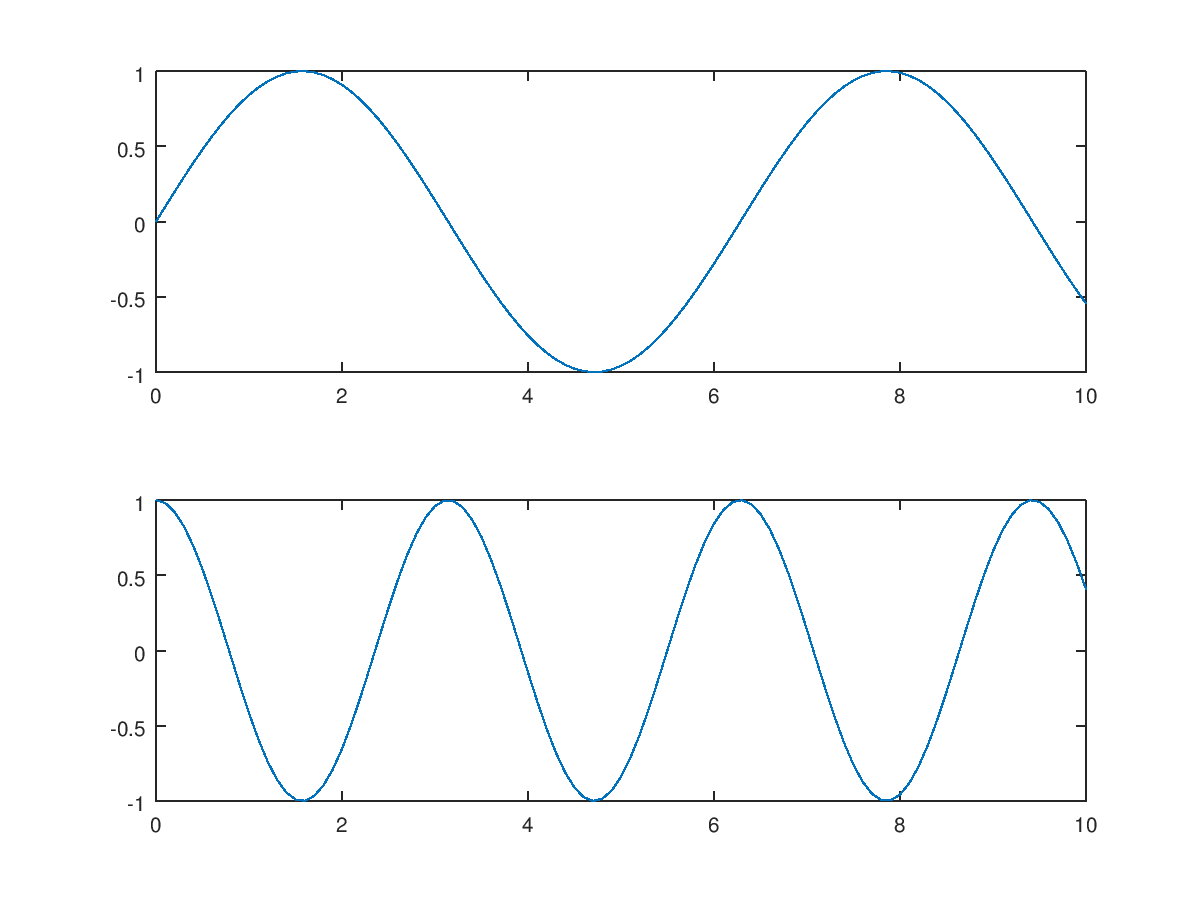
4. Splitting plots

   Plot sin(t) and cos(2t) graphs, with sin(t) on the top and cos(2t) at the bottom:

   t=0:0.1:10;
   x=sin(t);
   y=cos(2*t);
   subplot(211); plot(t,x);   % 2 rows 1 column, first graph
   subplot(212); plot(t,y);   % 2 rows 1 column, second graph
   

   The result is as follows:

   

Exercise 2

Plot three graphs, arranged top to middle to bottom, in order: $\cos(100\pi t)$, $\cos(1000\pi t)$, and $\cos(100\pi t)\cos(1000\pi t)$ (Note: $\pi$ can be directly represented by pi).