Python 采样

Python 有很多套件可用，其中对于数据处理的部份，numpy 和 matplotlib 都是常被使用的套件，前者可用来处理各种矩阵运算，后者可以用来画图，这两个合起来，可以执行很多 MATLAB/Octave 程式的功能，而且语法非常相似。

我们一样假设信号频率为9，然后分别用采样频率100和10来观察信号采样的结果。程式码如下：

import numpy as np
import matplotlib.pyplot as plt

# Define the time vector for one second duration
t = np.arange(0, 1, 0.001)  # Time from 0 to 1 second with 1ms interval

# Define the frequency of the cosine wave
f = 9  # Frequency of 9 Hz

# Generate the cosine wave
cosine_wave = np.cos(2 * np.pi * f * t)

# Plot the original cosine wave
plt.figure()
plt.subplot(3, 1, 1)
plt.plot(t, cosine_wave)
plt.title('Original Cosine Wave (9 Hz)')

# Sample the cosine wave at 100 Hz
fs1 = 100  # Sampling rate of 100 Hz
n1 = np.arange(0, 1, 1/fs1)  # Sample times
samples1 = np.cos(2 * np.pi * f * n1)

# Plot the sampled signal at 100 Hz
plt.subplot(3, 1, 2)
plt.stem(n1, samples1, 'r', markerfmt='ro', basefmt=" ")
plt.title('Sampled at 100 Hz')

# Sample the cosine wave at 10 Hz
fs2 = 10  # Sampling rate of 10 Hz
n2 = np.arange(0, 1, 1/fs2)  # Sample times
samples2 = np.cos(2 * np.pi * f * n2)

# Plot the sampled signal at 10 Hz
plt.subplot(3, 1, 3)
plt.stem(n2, samples2, 'g', markerfmt='go', basefmt=" ")
plt.title('Sampled at 10 Hz')

# Show the results
plt.xlabel('Time (seconds)')
plt.ylabel('Amplitude')
plt.tight_layout()
plt.show()

执行结果如下：

Python Sampling

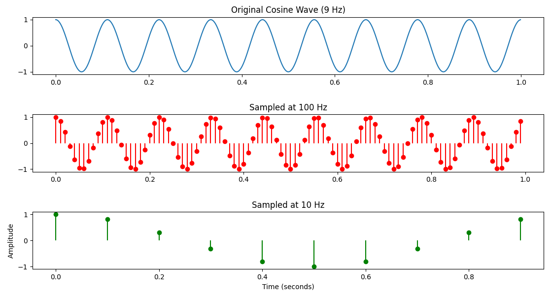
可以看到不管程式码，或者执行的结果，都和 Octave 的部份非常相似。

練習 4

练习安装上面所说的两个套件，并实际执行上述的程式码，观察结果是否相同。（建议用 Anaconda 或 venv 建立一个 Python 的执行环境，并用 pip install numpy matplotlib 安装套件）